7.2 Events

Posted on April 23, 2020 by user

7.2 Events

(A) Elements of a Sample Space which Satisfy Given Condition

When a specific condition is given, we can list the elements of a sample space which satisfy the given condition.

Example 1:

A two-digit number which is not more than 25 is chosen at random. List the elements of the sample space which satisfy each of the following conditions.

(a) A perfect square is chosen.

(b) A prime number is chosen.

Solution:

Sample space

= {10, 11, 12, 13, 14, 15, 16, 17, 18, 19, 20, 21, 22, 23, 24, 25}

(a)

A perfect square is chosen

= {16, 25}

(b)

A prime number is chosen

= {11, 13, 17, 19, 23}

(B) Events for a Sample Space

An event is a set of outcomes which satisfy a specific condition.

Event is a subset is a sample space.

Example 2:

A coin and a die are thrown simultaneously. The events P and Q are defined as follows.

P = Event of obtaining a ‘heads’ from the coin and an odd number from the die.

Q = Event of obtaining a ‘tails’ from the coin and a number more than 2 from the die.

(a) List the sample space, S.

(b) List the elements of

(i) The event P,

(ii) The event Q.

Solution:

(a)

Sample space, S

= { (H, 1), (H, 2), (H, 3), (H, 4), (H, 5), (H, 6), (T, 1), (T, 2), (T, 3), (T, 4), (T, 5), (T, 6) }

(b)(i)

P = { (H, 1), (H, 3), (H, 5) }

← (Set of outcomes of Event P: obtaining a ‘heads’ from the coin and an odd number from the die.)

(b)(ii)

Q = { (T, 3), (T, 4), (T, 5), (T, 6) }

← (Set of outcomes of Event Q: obtaining a ‘tails’ from the coin and a number more than 2 from the die.)

6.5 Cumulative Frequency

Posted on April 23, 2020 by user

6.5 Cumulative Frequency

Cumulative Frequency of a data or a class interval in a frequency table is obtained by determining the sum of its frequency with the total frequencies of all its previous data or class interval.

(A) Ogive

Ogive is a cumulative frequency graph which is obtained by plotting the cumulative frequency against the upper boundaries of each class.

Example:

The data below shows the number of books read by a group of 60 students in a year.

Books	Frequency
6-10	3
11-15	7
16-20	11
21-25	16
26-30	11
31-35	8
36-40	4

(a) Construct a cumulative frequency table for the given data.

(b) By using the scales of 2 cm to 5 books on the horizontal axis and 2 cm to 10 students on the vertical axis, draw an ogive for the data.

Solution:

(a)

Add a class with frequency 0 before the first class.
Find the upper boundary of each class interval.

Books	Frequency	Cumulative Frequency	Upper Boundary
1-5	0	0	5.5
6-10	3	0 + 3 = 3	10.5
11-15	7	3 + 7 = 10	15.5
16-20	11	10 + 11 = 21	20.5
21-25	16	21 + 16 = 37	25.5
26-30	11	37 + 11 = 48	30.5
31-35	8	48 + 8 = 56	35.5
36-40	4	56 + 4 = 60	40.5

(b)

6.7 SPM Practice (Long Questions)

Posted on April 23, 2020 by user

Question 3:

The data below shows the mass, in kg, of 50 students.

(a) Copy and complete the table below based on the data above.

(b) Based on the completed table above,

(i) State the size of the class interval used in the table.

(ii) Calculate the estimated mean of the mass of the students.

For this part of the question, use graph paper.
(c) By using a scale of 2 cm to 5 kg on the horizontal axis and 2 cm to 2 students on the vertical axis, draw a frequency polygon for the data.

Solution:
(a)

(b)(i)

Size of class interval

= upper boundary – lower boundary

= 44.5 – 39.5

= 5

(b)(ii)

\begin{array}{l} Estimated mean = \frac{42 \times 4 + 47 \times 9 + 52 \times 7 + 57 \times 9 + 62 \times 18 + 67 \times 3}{50} \\ = \frac{2785}{50} = 55.7 \end{array}

(c)

6.1 Class Intervals

Posted on April 23, 2020 by user

6.1 Class Interval

1. Data that consist of the measurement of a quantity can be grouped into few classes and the range of each class in known as the class interval.

(A) Class Limits and Boundaries

Lower Limit and Upper Limit

2. For class interval, for example 30 – 39, the smaller value (30) is known as the lower limit while the larger value (39) is known as the upper limit.

Lower Boundary and Upper Boundary

3. The lower boundary of a class interval is the middle value between the lower limit of the class interval and the upper limitof the class before it.

4. The upper boundary of a class interval is the middle value between the upper limit of the class interval and the lower limitof the class after it.

Example:

20 – 29

30 – 39

40 – 49

\begin{array}{l} Lower boundary of the class 30 - 39 \\ = \frac{29 + 30}{2} = 29.5 \\ Upper boundary of the class 30 - 39 \\ = \frac{39 + 40}{2} = 39.5 \end{array}

(B) Class size

5. The class size is the difference between the upper boundary and the lower boundary of the class.

Example:

Size of class interval 30 – 39

= Upper boundary – Lower boundary

= 39.5 – 29.5

= 10

6.3 Histograms

Posted on April 23, 2020 by user

6.3 Histograms

(A) Draw a histogram based on the frequency table of a grouped data

1. A histogram is a graphical representation of a frequency distribution.

2. A histogram consists of vertical rectangular bars without any spacing between them.

3. Steps for drawing a histogram

(a) Determine the lower boundaries and upper boundaries for each class interval.

(b) Choose suitable scales for the horizontal axis (x-axis) to represent class interval and the vertical axis (y-axis) to represent frequency.

Example:

The following frequency table shows the radii, in cm, of different types of trees in a garden.

Radii (cm)	Frequency
2.0 – 2.4	7
2.5 – 2.9	5
3.0 – 3.4	10
3.5 – 3.9	2
4.0 – 4.4	6
4.5 – 4.9	4

Draw a histogram to represent the above information.

Solution:

Radii (cm)	Frequency	Lower boundary	Upper boundary
2.0 – 2.4	7	1.95	2.45
2.5 – 2.9	5	2.45	2.95
3.0 – 3.4	10	2.95	3.45
3.5 – 3.9	2	3.45	3.95
4.0 – 4.4	6	3.95	4.45
4.5 – 4.9	4	4.45	4.95

6.7 SPM Practice (Long Questions)

Posted on April 23, 2020 by user

Question 1:

The data below shows the age of 25 tourists who visited a tourist spot.

(a) Copy and complete the table below based on the data above.

(b) Based on the completed table above,

(i) State the modal class.

(ii) Calculate the mean age of the tourists.

(c) For this part of the question, use graph paper.

By using a scale of 2 cm to 5 years on the horizontal axis and 2 cm to 1 tourist on the vertical axis, draw a histogram for the data.

Solution:
(a)

Calculation of midpoint for (age 6 – 10) =

\frac{6 + 10}{2} = 8

(b)(i)
Modal class = age 16 – 20 (highest frequency)

(b)(ii)

\begin{array}{l} mean age = \frac{3 \times 2 + 8 \times 5 + 13 \times 3 + 18 \times 8 + 23 \times 3 + 28 \times 4}{25} \\ = 16.4 \end{array}

(c)

6.6 Measures of Dispersion (Part 1)

Posted on April 23, 2020 by user

6.6 Measures of Dispersion

(A) Determine the range of a set of data

1. For an ungrouped data,

Range = largest value – smallest value.

2. For a grouped data,

Range = midpoint of the last class – midpoint of the first class.

Example 1:

Determine the range of the following data.

(a) 720, 840, 610, 980, 900

(b)

Time (minutes)	1 – 6	7 – 12	13 – 18	19 – 24	25 – 30
Frequency	3	5	9	4	4

Solution:

(a)

Largest value of the data = 980

Smallest value of data = 610

Range = 980 – 610 = 370

(b)

Midpoint of the last class

= ½ (25 + 30) minutes

= 27.5 minute

Midpoint of the first class

= ½ (1 + 6) minutes

= 3.5 minute

Range = (27.5 – 3.5) minute = 24 minutes

6.4 Frequency Polygons

Posted on April 23, 2020 by user

6.4 Frequency Polygons

1. A frequency polygon is a line graph that connects the midpoints of each class interval at the top end of each rectangle in a histogram.

2. A frequency polygon can be drawn from a

(a) Histogram,

(b) Frequency table

3. Steps for drawing a frequency polygon:

Step 1: Add a class with 0 frequency before the first class and add also a class with 0 frequency after the last class.

Step 2: Calculate the midpoints or mark the midpoints of the top sides of the rectangular bars including the midpoints of the two additional classes.

Step 3: Joint all the midpoints with straight lines.

Example:

The following frequency table shows the distance travelled by 38 teenagers by motorcycles in one afternoon.

Journey travelled (km)	Frequency
55 – 59	4
60 – 64	4
65 – 69	7
70 – 74	8
75 – 79	9
80 – 84	6

Draw a frequency polygon based on the frequency table.

Solution:

Journey travelled (km)	Frequency	Midpoint
50 – 54	0	52
55 – 59	4	57
60 – 64	4	62
65 – 69	7	67
70 – 74	8	72
75 – 79	9	77
80 – 84	6	82
85 – 89	0	87

6.2 Mode and Mean of Grouped Data

Posted on April 23, 2020 by user

6.2 Mode and Mean of Grouped Data

(A) Modal Class

The modal class of grouped data is the class interval in the frequency table with the highest frequency.

(B) Class Midpoint

The class midpoint is the value of data that lies at the centre of a class.

Class midpoint = \frac{Lower limit + Upper limit}{2}

(C) Calculating the Mean of Grouped Data

The steps to calculate the mean of grouped data are as follows.

Step 1: Calculate the midpoint value of each class.

Step 2: Calculate the value of (frequency × midpoint value) of each class.

Step 3: Calculate the sum of the values of (frequency × midpoint value) of all the classes.

Step 4: Calculate the sum of all the frequencies of all the classes.

Step 5: Calculate the value of the mean using the formula below.

\begin{array}{l} \begin{array}{l} Mean of grouped data, \bar{x} \\ = \frac{Sum of (frequency \times midpoint)}{Sum of frequencies} \\ = \frac{\sum f x}{\sum f} \\ Where Σ is the notation of summation, \\ x is the midpoint of a class and f is its frequency . \end{array} \end{array}

6.7 SPM Practice (Long Questions)

Posted on April 23, 2020 by user

Question 2:
Diagram below shows the marks, obtained by a group of 24 students in a mathematics quiz.

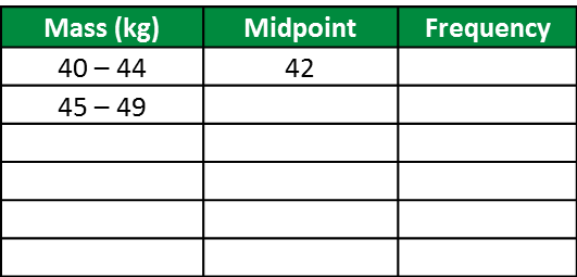
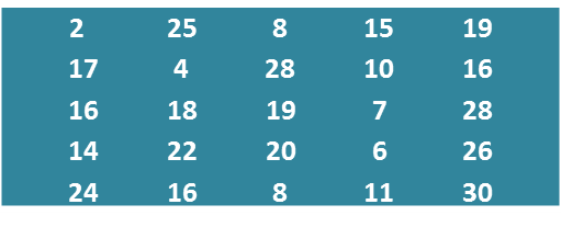
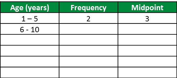
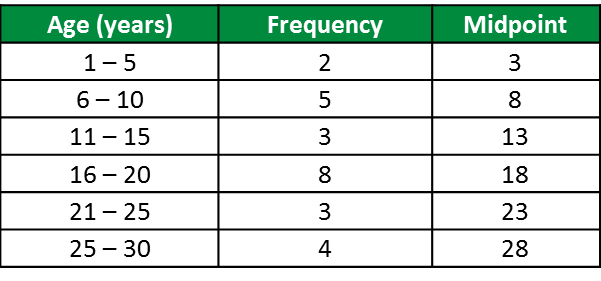
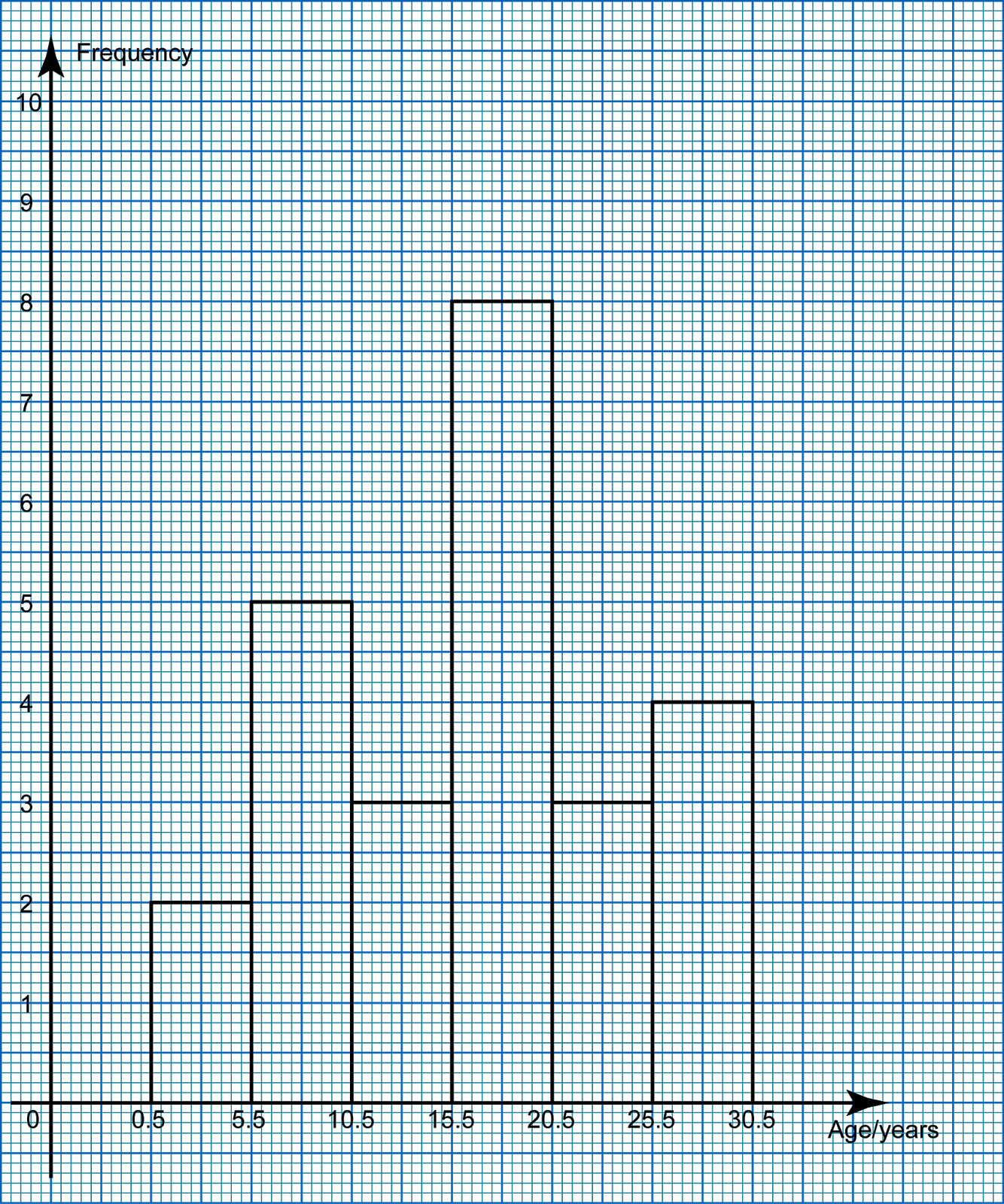
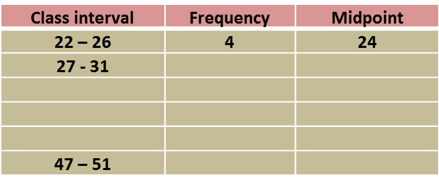
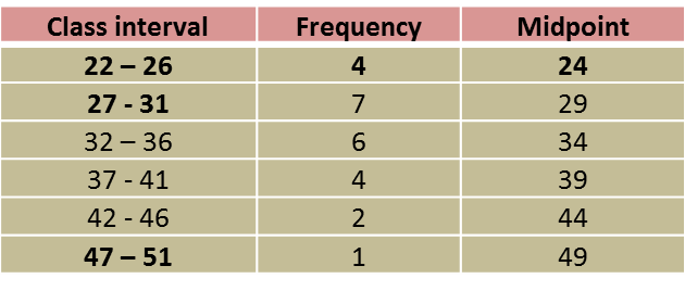
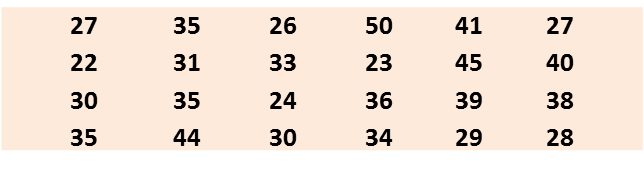
(a) Based on the data in diagram above, complete Table in the answer space.

(b) State the modal class.

(c) Calculate the estimated marks obtained by a student.

(d) For this part of the question, use graph paper.
By using a scale of 2 cm to 5 marks on the horizontal axis and 2 cm to 1 student on the vertical axis, draw a histogram for the data.

(e) Based on the histogram drawn in (d), state the number of students who obtain less than 32 marks in the quiz.

Answer:

Solution:
(a)

(b) Modal class = 27 – 31 (highest frequency)

\begin{array}{l} (c) \\ Estimated mean \\ = \frac{4 \times 24 + 7 \times 29 + 6 \times 34 + 4 \times 39 + 2 \times 44 + 1 \times 49}{24} \\ = \frac{796}{24} \\ = 33.17 marks \end{array}

(d)

(e)
Number of students who obtained less than 32 marks
= 4 + 7
= 11