Short Questions (Question 1 & 2)

Posted on April 21, 2020 by user

Question 1:

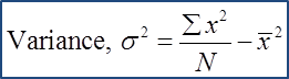
Given that the standard deviation of five numbers is 6 and the sum of the squares of these five numbers is 260. Find the mean of this set of numbers.

Solution:

\begin{array}{l} Given that σ = 6, Σ x^{2} = 260. \\ σ = 6 \\ \sqrt{\frac{Σ x^{2}}{n} - {\bar{X}}^{2}} = 6 \\ \frac{Σ x^{2}}{n} - {\bar{X}}^{2} = 36 \\ \frac{260}{5} - {\bar{X}}^{2} = 36 \\ {\bar{X}}^{2} = 16 \\ \bar{X} = \pm 4 \\ ∴ mean = \pm 4 \end{array}

Question 2:
Both of the mean and the standard deviation of 1, 3, 7, 15, m and n are 6. Find

(a) the value of m + n,

(b) the possible values of n.

Solution:

(a)

\begin{array}{l} Given mean = 6 \\ \frac{Σ x}{n} = 6 \\ \frac{Σ x}{6} = 6 \end{array}

1 + 3 + 7 + 15 + m + n= 36

26 + m + n= 36

m + n = 10

(b)

\begin{array}{l} σ = 6 \\ σ^{2} = 36 \\ \frac{Σ x^{2}}{n} - {\bar{X}}^{2} = 36 \\ \frac{1 + 9 + 49 + 225 + m^{2} + n^{2}}{6} - 6^{2} = 36 \\ \frac{284 + m^{2} + n^{2}}{6} - 36 = 36 \\ \frac{284 + m^{2} + n^{2}}{6} = 72 \\ 284 + m^{2} + n^{2} = 432 \\ m^{2} + n^{2} = 148 \\ From (a), m = 10 - n \\ {(10 - n)}^{2} + n^{2} = 148 \\ 100 - 20 n + n^{2} + n^{2} = 148 \\ 2 n^{2} - 20 n - 48 = 0 \\ n^{2} - 10 n - 24 = 0 \\ (n - 6) (n + 4) = 0 \\ n = 6 or - 4 \end{array}

Measures of Dispersion (Part 3)

Posted on April 21, 2020 by user

Measures of Dispersion (Part 3)
7.3 Variance and Standard Deviation

1. The variance is a measure of the mean for the square of the deviations from the mean.

2. The standard deviation refers to the square root for the variance.

(A) Ungrouped Data

Example 1:

Find the variance and standard deviation of the following data.

15, 17, 21, 24 and 31

Solution:

\begin{array}{l} Variance, σ^{2} = \frac{\sum x^{2}}{N} - {\bar{x}}^{2} \\ σ^{2} = \frac{15^{2} + 17^{2} + 21^{2} + 24^{2} + 31^{2}}{5} \\ - {(\frac{15 + 17 + 21 + 24 + 31}{5})}^{2} \\ σ^{2} = \frac{2492}{5} - {21.6}^{2} \\ σ^{2} = 31.84 \\ Standard deviation, σ = \sqrt{variance} \\ σ = \sqrt{31.84} \\ σ = 5.642 \end{array}

(B) Grouped Data (without Class Interval)

Example 2:

The data below shows the numbers of children of 30 families:

Number of child	2	3	4	5	6	7	8
Frequency	6	8	5	3	3	3	2

Find the variance and standard deviation of the data.

Solution:

\begin{array}{l} Mean \bar{x} = \frac{\sum f x}{\sum f} \\ = \frac{(6) (2) + (8) (3) + (5) (4) + (3) (5) + (3) (6) + (3) (7) + (2) (8)}{6 + 8 + 5 + 3 + 3 + 3 + 2} \\ = \frac{126}{30} = 4.2 \\ \frac{\sum f x^{2}}{\sum f} \\ = \frac{(6) {(2)}^{2} + (8) {(3)}^{2} + (5) {(4)}^{2} + (3) {(5)}^{2} + (3) {(6)}^{2} + (3) {(7)}^{2} + (2) {(8)}^{2}}{6 + 8 + 5 + 3 + 3 + 3 + 2} \\ = \frac{634}{30} = 21.13 \\ Variance, σ^{2} = \frac{\sum f x^{2}}{\sum f} - {\bar{x}}^{2} \\ σ^{2} = 21.133 - {4.2}^{2} \\ σ^{2} = 3.493 \\ Standard deviation, σ = \sqrt{variance} \\ σ = \sqrt{3.493} \\ σ = 1 .869 \end{array}

(C) Grouped Data (with Class Interval)

Example 3:

Daily Salary(RM)	Number of workers
10 – 14	40
15 – 19	25
20 – 24	15
25 – 29	12
30 – 34	8

Find the mean of daily salary and its standard deviation.

Solution:

Daily Salary (RM)	Number of workers, f	Midpoint, x	fx	fx²
10 – 14	40	12	480	5760
15 – 19	25	17	425	7225
20 – 24	15	22	330	7260
25 – 29	12	27	324	8748
30 – 34	8	32	256	8192
Total	100		1815	37185

\begin{array}{l} Mean \bar{x} = \frac{\sum f x}{\sum f} \\ Mean of daily salary = \frac{1815}{100} = 18.15 \\ Variance, σ^{2} = \frac{\sum f x^{2}}{\sum f} - {\bar{x}}^{2} \\ Standard deviation, σ = \sqrt{variance} \\ σ^{2} = \frac{37185}{100} - {18.15}^{2} \\ σ^{2} = 42.43 \\ σ = \sqrt{42.43} \\ σ = 6 .514 \end{array}

Measures of Dispersion (Part 2)

Posted on April 21, 2020 by user

Measures of Dispersion (Part 2)
7.2b Interquartile Range 2

(C) Interquartile Range of Grouped Data (with Class Interval)

The interquartile range of grouped data can be determined by Method 1 (using a cumulative frequency table) or Method 2 (using an ogive).

Example:
The table below shows the marks obtained by a group of Form 4 students in school mathematics test.

Estimate the interquartile range.

Solution:

Method 1: From Cumulative Frequency Table

Step 1:

Lower quartile, Q₁= the

\frac{1}{4} {(60)}^{th}

observation

= the 15^thobservation

Upper quartile, Q₃= the

\frac{3}{4} {(60)}^{th}

observation
= the 45^thobservation

Step 2:

\begin{array}{l} Lower quartile, Q_{1} = L_{1} + (\frac{\frac{1}{4} N - F_{1}}{f_{Q_{1}}}) C \\ = 39.5 + (\frac{15 - 12}{20}) 10 \\ = 39.5 + 1.5 \\ = 41 \end{array}

Step 3:

\begin{array}{l} Upper quartile, Q_{3} = L_{3} + (\frac{\frac{3}{4} N - F_{3}}{f_{Q_{3}}}) C \\ = 49.5 + (\frac{45 - 32}{16}) 10 \\ = 49.5 + 8.125 \\ = 57.625 \end{array}

Step 4:

Interquartile Range

= upper quartile – lower quartile

= Q₃– Q₁

= 57.625 – 41

= 16.625

Measures of Dispersion (Part 2)

Posted on April 21, 2020 by user

Measures of Dispersion (Part 2)
7.2b Interquartile Range 1

(A) Interquartile Range of Ungrouped Data

Example 1:

Find the interquartile range of the following data.

(a) 7, 5, 1, 3, 6, 11, 8

(b) 12, 4, 6, 18, 9, 16, 2, 14

Solution:
(a) Rearrange the data according to ascending order.

Interquartile Range

= upper quartile – lower quartile

= 8 – 3

= 5

(b) Rearrange the data according to ascending order.

Interquartile Range

= upper quartile – lower quartile

\frac{14 + 16}{2} - \frac{4 + 6}{2}

= 15 – 5
= 10

(B) Interquartile Range of Grouped Data (without Class Interval)

Example 2:

The table below shows the marks obtained by a group of Form 4 students in school mid-term science test.

Determine the interquartile range of the distribution.

Solution:

Lower quartile, Q₁= the

\frac{1}{4} {(24)}^{th}

observation

= the 6^thobservation

= 2

Upper quartile, Q₃= the

\frac{3}{4} {(24)}^{th}

observation

= the 18^thobservation

= 4

Interquartile Range

= upper quartile – lower quartile

= Q₃– Q₁

= 4 – 2

= 2

Measures of Dispersion (Part 1)

Posted on April 21, 2020 by user

Measures of Dispersion (Part 1)

7.2a Range

(A) Range of Ungrouped Data

Example 1:
Find the range for the set of data 2, 4, 7, 10, 13, 16 and 18.

Solution:

Range = largest value – smallest value

= 18 – 2

= 16

(B) Range of Grouped Data (with Class Interval)

Example 2:

The grouped frequency distribution was obtained from 100 students regarding the scores in their test shown as below.

Find the range of the data.

Solution:

\begin{array}{l} Range \\ = midpoint of the highest class - midpoint of the lowest class \\ Range = \frac{35 + 39}{2} - \frac{5 + 9}{2} \\ = 37 - 7 \\ = 30 \end{array}

7.1c Median

Posted on April 21, 2020 by user

7.1c Median

1. The median of a group of data refers to the value which is at the middle of the data after the data has been arranged according to grouped data and ungrouped data.

(A) Ungrouped Data

Example 1:

Find the median for each of the sets of data given below.

(a) 15, 18, 21, 25, 20, 18

(b) 13, 6, 9, 17, 11

Solution:
(a) Arrange the data in the ascending order

15, 18, 18, 20, 21, 25

Median = T_{\frac{n + 1}{2}} = T_{\frac{6 + 1}{2}} = T_{3 \frac{1}{2}} = \frac{18 + 20}{2} = 19

(b) 6, 9, 11, 13, 17

Median = T_{\frac{n + 1}{2}} = T_{\frac{5 + 1}{2}} = T_{3} = 11

(B) Grouped Data (without Class Interval)

Example 2:

The frequency table shows the marks obtained by 40 students in a biology test.

Solution:

Median = T_{\frac{n + 1}{2}} = T_{\frac{40 + 1}{2}} = T_{20 \frac{1}{2}} = 60 \leftarrow (20 \frac{1}{2} th term is 60)

(C) Grouped Data (with Class Interval)

m = median

L = Lower boundary of median class

N = Number of data

F = Total frequency before median class

f_m = Total frequency in median class

c = Class size = (Upper boundary – lower boundary)

1. The median can be determined from an accumulative frequency table and the ogive.

2. The ogive is an accumulative graph; the median, quartiles and the range between quartiles can be determined from it.

Example 3:

The grouped frequency distribution was obtained from 100 students regarding the scores in their test shown as below.

Find the median.

Solution:
Method 1: using formula

\begin{array}{l} S t e p 1 \\ Median class is given by T_{\frac{n}{2}} = T_{\frac{100}{2}} = T_{50} \\ ∴ Median class is the class 20 - 24 \\ S t e p 2 \\ m = L + (\frac{\frac{N}{2} - F}{f_{m}}) c \\ m = 19.5 + (\frac{\frac{100}{2} - 33}{26}) 5 \\ m = 19.5 + 3.269 = 22.77 \end{array}

7.1b Mode

Posted on April 21, 2020 by user

7.1b Mode

Mode is the observation which has the highest frequency in a set of data.

Example:

Find the mode for each of the sets of data given below.

(a) 15, 18, 21, 25, 20, 18

(b) 3, 6, 9, 11, 17

(c) 0, 1, 2, 7, 3, 2, 1, 1, 2, 1, 2

Solution:

(a) The mode is 18. ← (18 occurs 2 times)

(b) Does not have a mode.

(c) The modes are 1 and 2. ← (Both numbers occur 4 times)

7.1a Mean

Posted on April 21, 2020 by user

7.1a Mean
1. The mean of the data is an average value obtained by using the formula:
Mean= Total data values Number of data

(A) Ungrouped Data

Example 1

(a) Find the mean for the set of data 2, 4, 7, 10, 13, 16 and 18.

(b) A value of xis added into the above set of data, the mean for this new data is 9.5. Determine the value of x.

Solution:
(a)

\begin{array}{l} \bar{x} = \frac{2 + 4 + 7 + 10 + 13 + 16 + 18}{7} \\ \bar{x} = \frac{70}{7} = 10 \end{array}

(b)

\begin{array}{l} New mean = 9.5 \\ \frac{70 + x}{8} = 9.5 \\ 70 + x = 76 \\ x = 6 \end{array}

(B) Grouped Data (Without Class Interval)

Example 2

The frequency table shows the marks obtained by 40 students in a Biology test.

Find the mean marks.

Solution:

\begin{array}{l} Mean marks, \bar{x} \\ \bar{x} = \frac{(50) (6) + (55) (8) + (60) (15) + (65) (10) + (70) (1)}{6 + 8 + 15 + 10 + 1} \\ \bar{x} = \frac{2360}{40} = 59 \end{array}

(C) Grouped Data (With Class Interval)

Example 3

The grouped frequency distribution was obtained from 100 students regarding the scores in their test shown as below.

Find the mean scores.

Solution:

\begin{array}{l} Mid-point = \frac{5 + 9}{2} = 7 \\ Mean scores, \bar{x} = \frac{\sum f x}{\sum f} = \frac{2290}{100} = 22.9 \end{array}

Long Questions (Question 4)

Posted on April 21, 2020 by user

Question 4:
Solutions by scale drawing will not be accepted.
Diagram below shows a triangle PRS. Side PR intersects the y-axis at point Q.

(a) Given PQ : QR = 2 : 3, find
(i) The coordinates of P,
(ii) The equation of the straight line PS,
(iii) The area, in unit², of triangle PRS.
(b) Point M moves such that its distance from point R is always twice its distance from point S.
Find the equation of the locus M.

Solution:
(a)(i)

\begin{array}{l} P = (\frac{2 (6) + 3 h}{2 + 3}, \frac{2 (12) + 3 k}{2 + 3}) \\ (0, 6) = (\frac{12 + 3 h}{5}, \frac{24 + 3 k}{5}) \\ \frac{12 + 3 h}{5} = 0 \\ 3 h = - 12 \\ h = - 4 \\ \frac{24 + 3 k}{5} = 6 \\ 3 k = 30 - 24 \\ k = 2 \\ P = (- 4, 2) \end{array}

(a)(ii)

\begin{array}{l} m_{P S} = \frac{2 - (- 6)}{- 4 - 2} \\ = - \frac{8}{6} \\ = - \frac{4}{3} \\ Equation of P S : \\ y - y_{1} = - \frac{4}{3} (x - 2) \\ y - (- 6) = - \frac{4}{3} x + \frac{8}{3} \\ 3 y + 18 = - 4 x + 8 \\ 3 y = - 4 x - 10 \end{array}

(a)(iii)

\begin{array}{l} Area of △ P R S \\ = \frac{1}{2} | \begin{array}{l} - 4      2       6 \\ 2 - 612 \end{array} \begin{array}{l} - 4 \\ 2 \end{array} | \\ = \frac{1}{2} | (24 + 24 + 12) - (4 - 36 - 48) | \\ = \frac{1}{2} | 60 - (- 80) | \\ = 70 {unit}^{2} \end{array}

(b)

\begin{array}{l} Let P = (x, y) \\ M R = 2 M S \\ \sqrt{{(x - 6)}^{2} + {(y - 12)}^{2}} = 2 \sqrt{{(x - 2)}^{2} + {(y + 6)}^{2}} \\ {(x - 6)}^{2} + {(y - 12)}^{2} = 4 [{(x - 2)}^{2} + {(y + 6)}^{2}] \\ x^{2} - 12 x + 36 + y^{2} - 24 y + 144 = 4 [x^{2} - 4 x + 4 + y^{2} + 12 y + 36] \\ x^{2} - 12 x + y^{2} - 24 y + 180 = 4 x^{2} - 16 x + 4 y^{2} + 48 y + 160 \\ 3 x^{2} + 3 y^{2} - 4 x + 72 y - 20 = 0 \end{array}

Long Questions (Question 3)

Posted on April 21, 2020 by user

Question 3:

The diagram shows a triangle LMN where L is on the y-axis. The equation of the straight line LKN and MK are 2y – 3x + 6 = 0 and 3y + x– 13 = 0 respectively. Find

(a) the coordinates of K

(b) the ratio LK:KN

Solution:
(a)

2y – 3x + 6 = 0 ----(1)

3y + x – 13 = 0 ----(2)

x = 13 – 3y ----(3)

Substitute equation (3) into (1),

2y – 3 (13 – 3y) + 6 = 0

2y – 39 + 9y + 6 = 0

11y = 33

y = 3

Substitute y = 3 into equation (3),

x = 13 – 3 (3)

x = 4

Coordinates of K = (4, 3).

(b)

Given equation of LKN is 2y – 3x + 6 = 0

At y – axis, x = 0,

x coordinates of point L = 0.

\begin{array}{l} Ratio L K : K N \\ Equating the x coordinates, \\ \frac{L K (10) + K N (0)}{L K + K N} = 4 \\ 10 L K = 4 L K + 4 K N \\ 6 L K = 4 K N \\ \frac{L K}{K N} = \frac{4}{6} \\ \frac{L K}{K N} = \frac{2}{3} \\ Ratio L K : K N = 2 : 3 \end{array}